
Module 5 – Spreadsheets
Lesson 5 – Formatting and Data Presentation
Formatting makes spreadsheet data easier to read, understand and present. In this lesson you will work with number formats, cell formatting, borders, shading, resizing, headings, conditional formatting, freeze panes and alignment tools.
1. Number Formatting
Number formats change how values look without changing the value stored in the cell.
- General – default format.
- Number – allows decimal places.
- Currency – displays symbols such as £ or $.
- Accounting – aligns currency symbols neatly.
- Percentage – multiplies by 100 and adds %.
- Date – displays as day/month/year.
- Time – displays hours and minutes.
Examples:
- 0.25 → 25% (Percentage format)
- 1200 → £1,200.00 (Currency format)

- Type 0.2 into a cell.
- Change the format to Percentage.
- Change the format to Currency.
What differences do you notice?
Quick check: If you want to show 0.35 as 35%, which format should you use?
Use the Percentage format.
2. Cell Formatting
Cell formatting changes how the content appears inside a cell.
- Font type and size.
- Bold, italic, underline.
- Text colour.
- Cell background (fill colour).
- Alignment (left, centre, right).
- Wrap Text – keeps long text visible on multiple lines.

- Type a heading such as Monthly Sales Report into one cell.
- Apply bold, increase the font size and change the text colour.
- Turn on Wrap Text and make the column narrower.
3. Borders and Shading
Borders and shading help separate and highlight parts of your data.
- Add borders to cells or entire tables.
- Use thicker borders for titles or totals.
- Use shading to highlight key information.
- Use light colours for better readability.

Quick question: Where would a thick border be most useful?
Around totals or main headings so they stand out.
4. Adjusting Column Widths and Row Heights
You can make cells bigger or smaller to fit the data.
- Drag the boundary between column letters to resize columns.
- Double-click a column boundary to AutoFit width.
- Adjust row height for wrapped or larger text.

- Type a long text label into a cell.
- First, adjust the column width until all text fits on one line.
- Then turn on Wrap Text and reduce the column width.
Which layout looks clearer to you?
5. Formatting Headings
Headings help users understand what each column or row represents.
- Use bold text for headings.
- Increase font size for the heading row.
- Apply a fill colour to the heading row.
- Centre headings if required.

Quick check: Why is it useful to format headings differently from data?
It makes the headings easy to spot and helps users understand the structure of the data quickly.
6. Conditional Formatting (Basic)
Conditional formatting automatically changes how cells look based on rules.
You can use it to:
- Highlight values greater than a chosen number.
- Identify the highest or lowest values.
- Highlight duplicate values.
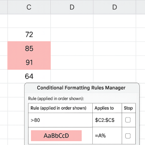
- Create a list of 10 numbers (for example, test scores).
- Use Conditional Formatting → Highlight Cells Rules → Greater Than….
- Highlight all scores above 70 in a light green colour.
7. Freeze Panes
Freeze panes keep important headings visible while you scroll.
Options include:
- Freeze Top Row – keeps the first row visible.
- Freeze First Column – keeps the first column visible.
- Freeze both top row and first column (using a selected cell).

Quick question: When is Freeze Panes most useful?
When working with large tables so you can still see headings while scrolling through the data.
8. Hide and Unhide Rows/Columns
You can temporarily hide data without deleting it.
- Hide columns containing extra detail.
- Hide rows you do not need to view right now.
- Right-click on a row/column header → Hide or Unhide.

9. Cell Alignment Options
Alignment affects where text appears inside a cell.
- Horizontal alignment: left, centre, right.
- Vertical alignment: top, middle, bottom.
- Wrap Text for long entries.
- Merge & Centre – combine cells and centre text (best used for headings, avoid inside data tables).

Quick check: Why should you avoid “Merge & Centre” inside data tables?
It can break sorting and filtering and make formulas harder to manage.
10. Practical Activity
- Create a small table of sales data with headings such as Product, Units Sold, Price, Total.
- Format the heading row with bold text and a fill colour.
- Apply Currency format to the Price and Total columns.
- Resize columns so that all text is visible (use AutoFit).
- Apply Conditional Formatting to highlight Total values above a chosen amount.
- Use Freeze Top Row so headings stay visible while scrolling.
- Hide one column, then unhide it again.
::contentReference[oaicite:0]{index=0}