Advanced Spreadsheets – Lesson 1: Advanced Workbook and Data Setup

Learning Outcomes

By the end of this lesson, you will be able to:

• Organise worksheets clearly and professionally.
• Control how your workbook is displayed for easier navigation.
• Format numbers, dates and times using advanced options.
• Create and use templates for repeated workbooks.
• Enter data more efficiently using built-in tools.
• Set up a workbook in a structured, professional way.

1. Workbook and Worksheet Management

This section covers how to rename, insert, delete, move, copy, hide and colour worksheets so your workbook is easy to understand and navigate.

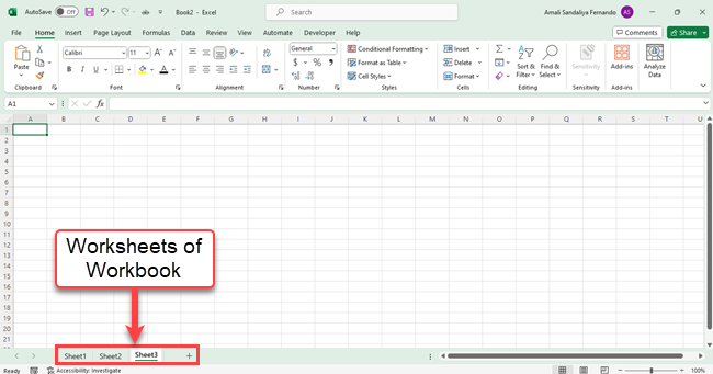
1.1 Renaming worksheets

Use clear, meaningful names so that anyone opening the workbook understands what each sheet contains.

1. Double-click the sheet tab at the bottom (for example, “Sheet1”).
2. Type a clear name, for example: Sales 2025 or Raw Data.
3. Press Enter to confirm.

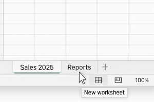
1.2 Inserting worksheets

Add new sheets when you need to separate different types of data or reports.

1. Click the + icon next to the existing sheet tabs.
2. A new sheet (for example, “Sheet2”) will appear.

1.3 Deleting worksheets

Delete sheets you no longer need, but be careful as this cannot always be undone.

1. Right-click the sheet tab you want to remove.
2. Click Delete.
3. Confirm if a warning message appears.

1.4 Moving worksheets

Reorder sheets so that related sheets sit next to each other.

1. Click and hold the sheet tab you want to move.
2. Drag it left or right to the new position.
3. Release the mouse button when you see a small black triangle showing the new position.

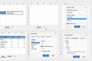
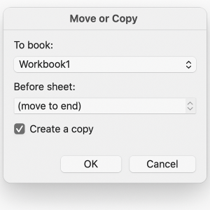
1.5 Copying worksheets

Copy a worksheet when you want the same layout or formulas but different data.

1. Right-click the sheet tab.
2. Click Move or Copy….
3. Tick Create a copy.
4. Choose the position in the list, or select another workbook (if one is open).
5. Click OK.

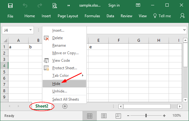
1.6 Hiding and unhiding worksheets

Hide sheets to keep supporting data out of the way, but still available for formulas.

To hide a sheet:

1. Right-click the sheet tab.
2. Click Hide.

To unhide a sheet:

1. Right-click any sheet tab.
2. Click Unhide….
3. Select the sheet name you want to show.
4. Click OK.

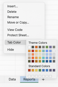
1.7 Changing worksheet tab colours

Use tab colours to group related sheets or highlight important ones.

1. Right-click the sheet tab.
2. Click Tab Colour.
3. Select a colour from the palette.

2. Workbook Display and Navigation

This section focuses on how to freeze headings, split the screen, and use different view settings to manage large sheets.

2.1 Freezing rows and columns (Freeze Panes)

Freeze panes keeps important headings visible while you scroll.

To freeze the top row:

1. Click anywhere on the sheet.
2. Go to View → Freeze Panes → Freeze Top Row.

To freeze the first column:

1. Click anywhere on the sheet.
2. Go to View → Freeze Panes → Freeze First Column.

To freeze both a row and a column:

1. Click the cell below the heading row and to the right of the heading column (for example, click B2 to freeze Row 1 and Column A).
2. Go to View → Freeze Panes → Freeze Panes.

To unfreeze panes: Go to View → Freeze Panes → Unfreeze Panes.

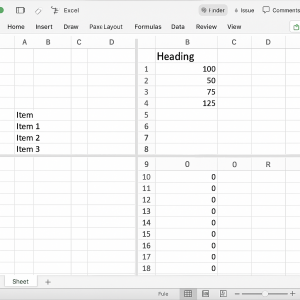
2.2 Splitting the window

Splitting the window allows you to see different parts of the same sheet at the same time.

1. Click in the cell where you want the split to start.
2. Go to View → Split.
3. Drag the split bars if needed.
4. To remove the split, click View → Split again.

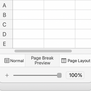
2.3 Zoom and worksheet views

Use zoom and view modes to control how your sheet appears on screen.

• Zoom: Use the slider in the bottom right corner, or go to View → Zoom.
• Normal View: Standard worksheet view.
• Page Break Preview: Shows where the page breaks occur when printing.
• Page Layout: Shows how the sheet will look on printed pages, including margins and headers.

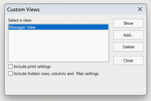
2.4 Custom views (where supported)

Custom views allow you to save display settings such as filters, hidden rows and zoom level.

1. Set up the sheet the way you want to see it (filters, zoom, hidden rows/columns).
2. Go to View → Custom Views.
3. Click Add…, give the view a name (for example, Manager View), and click OK.
4. To apply a view later, open Custom Views, select it, and click Show.
5. To remove a view, select it and click Delete.

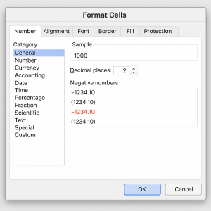
3. Advanced Cell and Number Formatting

This section explains how to use the Format Cells dialog to control the appearance of numbers, dates and times.

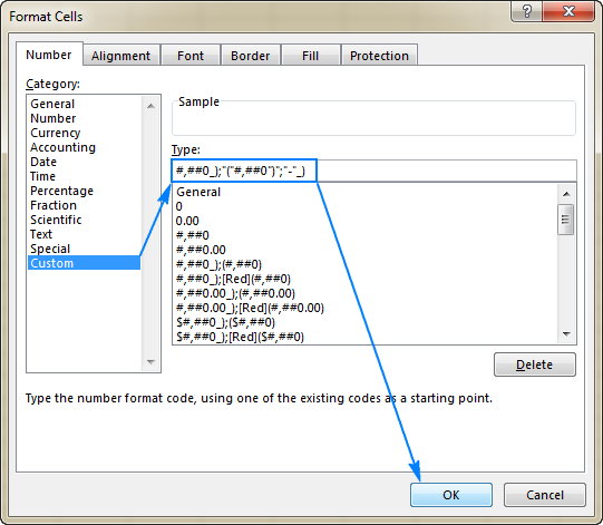
3.1 Opening the Format Cells dialog

1. Select the cell or range of cells you want to format.
2. Right-click and choose Format Cells…
   or press Ctrl + 1 on the keyboard.

3.2 Custom number formats

Use the Custom category in the Format Cells dialog to create specific number formats.

• Thousands separator: #,##0 (displays 15000 as 15,000)
• Negative numbers in brackets: #,##0;(#,##0)

1. Select your numbers.
2. Open Format Cells and click the Number tab.
3. Choose Custom.
4. Enter the custom format in the Type box.
5. Click OK.

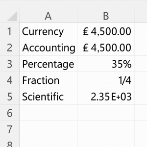
3.3 Common number formats

• Currency: Shows currency symbol and two decimal places (for example, £4,500.00).
• Accounting: Aligns currency symbols and decimal points neatly.
• Percentage: Converts 0.35 to 35%.
• Fraction: Shows values as fractions (for example, 0.25 as 1/4).
• Scientific: Shows numbers like 2,350 as 2.35E+03.

3.4 Date and time formats

Use clear, consistent formats for dates and times.

• dd-mmm-yyyy (for example, 12-Jan-2025)
• dd/mm/yyyy (for example, 12/01/2025)
• hh:mm for times (for example, 14:30)

1. Select date or time cells.
2. Open Format Cells.
3. Choose the Date or Time category, or use Custom for specific formats.
4. Click OK.

4. Working with Templates

Templates save time and ensure consistency across your workbooks.

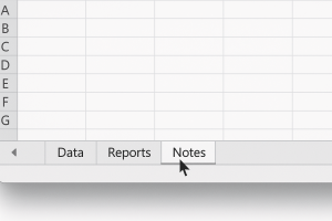
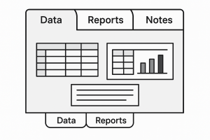
4.1 Creating a template workbook

1. Set up a workbook with standard sheet names (for example, Data, Reports, Notes).
2. Apply your preferred formatting, headings and formulas.
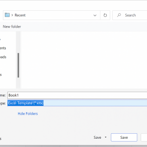
3. Go to File → Save As.
4. Select the location.
5. In the Save as type drop-down, choose Excel Template (*.xltx).
6. Give the template a clear name (for example, Monthly_Report_Template).
7. Click Save.

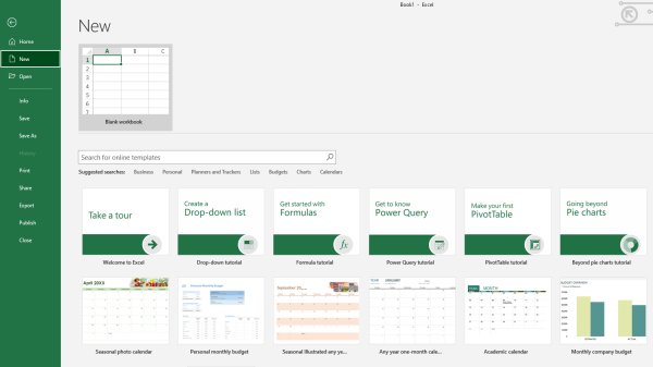
4.2 Creating a new workbook from a template

1. Go to File → New.
2. Choose Personal (or equivalent tab) to see your templates.
3. Click your template (for example, Monthly_Report_Template).
4. A new workbook based on that template will open.

4.3 Updating templates

Changes to a template will only affect new workbooks created from it, not existing workbooks.

1. Open the template file (.xltx) directly.
2. Make your changes (for example, new headings or formats).
3. Save the file again as a template.

5. Data Entry Efficiency

This section looks at tools such as Flash Fill, series fill and basic data validation lists to speed up data entry and reduce errors.

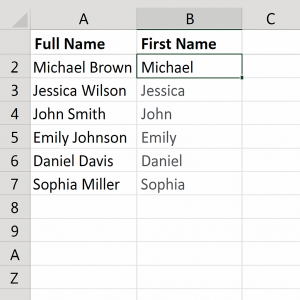
5.1 Using Flash Fill (where available)

Flash Fill recognises patterns in your data and completes the rest for you.

1. Enter your data in a column (for example, full names: “Alex Johnson”).
2. In the next column, type the result you want for the first row (for example, first name “Alex”).
3. Start typing the second result; Excel may suggest the rest.
4. Press Enter to accept the suggestion, or use Ctrl + E to apply Flash Fill.

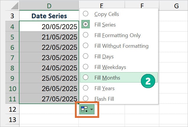
5.2 Using Fill Series for dates, times and lists

Use the fill handle to quickly create series.

1. Type the first value (for example, a date like 01/01/2025).
2. Drag the small square in the bottom-right corner of the cell (fill handle) down or across.
3. Release when you have the range you need.
4. Use the Auto Fill Options button (if shown) to adjust the pattern (for example, fill weekdays only).

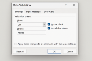
5.3 Basic data validation lists (drop-downs)

Data validation lists help restrict entries to valid options.

1. Select the cells where you want the drop-down list.
2. Go to Data → Data Validation.
3. In the Allow box, select List.
4. In the Source box, type your options separated by commas (for example, High,Medium,Low) or refer to a range with the options.
5. Click OK.

6. Good Practice for Advanced Workbooks

Follow these guidelines to keep complex workbooks clear and reliable.

• Use a separate sheet for raw data and another for reports.
• Keep headings and totals clearly separated from the main data table.
• Avoid typing totals manually; always use formulas linked to the data (for example, =SUM(B2:B50)).
• Document assumptions, versions and notes in a dedicated Notes sheet.
• Use clear sheet names and consistent formats throughout the workbook.

7. Practical Activity

Complete this activity to put the skills from this lesson into practice.

Task: Build a structured workbook and save it as a template

Step 1 – Create the workbook structure

1. Create a new Excel workbook.
2. Rename the first three sheets as:
   • Data
   • Reports
   • Notes

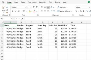
Step 2 – Add sample data and formatting on the Data sheet

1. On the Data sheet, create a small table with at least 5–10 rows. Use headings such as:
   • Date
   • Customer
   • Amount
   • Status
2. Format the Amount column using a custom currency format with thousands separators, for example £#,##0;(#,##0).
3. Format the Date column as dd-mmm-yyyy.
4. Use Data Validation to create a drop-down list in the Status column with options such as Paid,Unpaid,Pending.

Step 3 – Freeze panes on the Data sheet

1. Ensure your headings are in Row 1 and labels (if any) are in Column A.
2. Click cell B2.
3. Go to View → Freeze Panes → Freeze Panes to freeze the top row and first column.

Step 4 – Add notes on the Notes sheet

1. On the Notes sheet, type a short description of the workbook’s purpose. For example:
   • “This workbook is used to track monthly customer payments. Data is entered on the Data sheet, and summary reports will be built on the Reports sheet.”
2. Add any assumptions you are making (for example, “Amounts are entered in GBP only”).

Step 5 – Save the workbook as a template

1. Go to File → Save As.
2. Select your save location.
3. Choose Excel Template (*.xltx) as the file type.
4. Name the file Customer_Payments_Template.
5. Click Save.

Step 6 – Create a new workbook from your template

1. Close the workbook if it is still open.
2. Go to File → New.
3. Choose your Customer_Payments_Template template.
4. Confirm that the new workbook contains the Data, Reports and Notes sheets with the same structure and formatting.

Optional extension: On the Reports sheet, add a simple total using a formula such as =SUM(Data!C2:C50) to sum the Amount column from the Data sheet.