Advanced Spreadsheets
Lesson 3 – Logical and Conditional Functions
This lesson focuses on logical and conditional functions used to build decision-making formulas in a spreadsheet. You will work with IF, AND, OR, NOT, and the conditional summary functions SUMIF, SUMIFS, COUNTIF, COUNTIFS, AVERAGEIF and AVERAGEIFS.
1. Logical functions
Logical functions test conditions and return TRUE/FALSE or a result that you specify (such as Pass/Fail). They are often combined to build powerful decision rules.
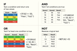
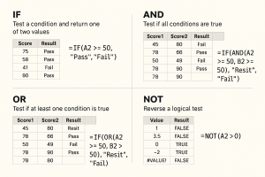
- IF – test a condition and return one of two values:
- =IF(A2 >= 50, “Pass”, “Fail”) – if the value in A2 is 50 or higher, return Pass, otherwise return Fail.
- AND – test if all conditions are true:
- =IF(AND(A2 >= 50, B2 >= 50), “Pass”, “Fail”) – only Pass if both scores are 50 or higher.
- OR – test if at least one condition is true:
- =IF(OR(A2 >= 50, B2 >= 50), “Resit”, “Fail”) – Resit if either score is 50 or higher, otherwise Fail.
- NOT – reverse a logical test:
- =NOT(A2 > 0) – returns TRUE if A2 is not greater than 0 (that is, A2 is 0 or negative).
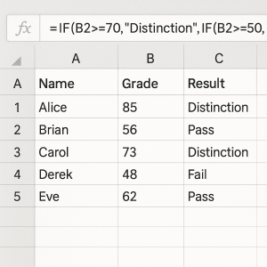
2. Nested IF statements
Nested IF formulas use one IF function inside another. This allows you to test several conditions in sequence and return different text or values.
- Use multiple IF functions inside a single formula to return more than two possible results.
- Example grading formula:
- =IF(B2 >= 70, “Distinction”, IF(A2 >= 50, “Pass”, “Fail”))
- The order of conditions is important – you must test the highest / most specific condition first, then move down in logical order.
- Keep nested IFs readable with clear spacing and indentation when possible.
3. Conditional summary functions
Conditional summary functions calculate totals or counts only for records that meet specified criteria. They are often used with structured tables or named ranges.
- SUMIF – sum values that meet a single condition:
- =SUMIF(Department, “Sales”, SalesTotal) – sums SalesTotal where Department is Sales.
- SUMIFS – sum values that meet multiple conditions:
- =SUMIFS(SalesTotal, Department, “Sales”, Month, “January”) – sums January SalesTotal for the Sales department only.
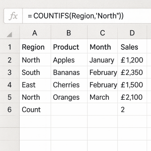
- COUNTIF – count cells that meet a single condition:
- =COUNTIF(Region, “North”) – counts how many records are in the North region.
- COUNTIFS – count cells that meet multiple conditions:
- Example: count orders for the North region in February only, using Region and Month ranges as criteria.
4. AVERAGEIF and AVERAGEIFS
AVERAGEIF and AVERAGEIFS work like SUMIF and SUMIFS but calculate an average instead of a total.
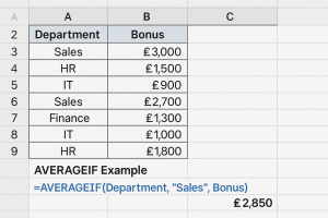
- AVERAGEIF – average numbers that meet a condition.
- AVERAGEIFS – average numbers that meet multiple conditions.
- Example:
- =AVERAGEIF(Department, “Sales”, Bonus) – averages the Bonus values for staff in the Sales department only.
5. Good practices with logical formulas
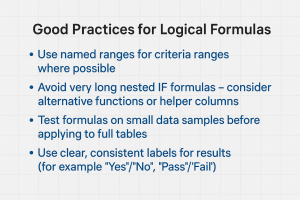
Logical formulas can become complex, so good design makes them easier to build, understand and maintain.
- Use named ranges for criteria ranges where possible (for example, Region, Department, SalesTotal).
- Avoid very long nested IF formulas – consider alternative functions such as IFS (where available), or use helper columns to break calculations into smaller steps.
- Test formulas on a small set of sample data before applying them to a large table.
- Use clear, consistent labels for results, such as “Yes”/”No” or “Pass”/”Fail”, so that reports are easy to read.
- Document any complex logic in a Notes sheet so other users understand how results are calculated.
6. Practical Activity
Complete this activity to apply the lesson skills.
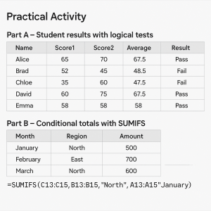
Part A – Student results with logical tests
- Create a student results table with the following columns: Name, Score1, Score2, Average, Result.
- In the Average column, use a formula such as =AVERAGE(B2:C2) to calculate each student’s average score.
- In the Result column, use an IF formula to label each student Pass or Fail based on the average (for example, Pass if average ≥ 50).
- Use AND or OR to apply additional conditions, such as requiring a minimum of 40 in each exam, even if the average is above 50.
Part B – Conditional totals with SUMIFS
- In the same workbook, or in a new sheet, create a small sales table with columns such as Month, Region, Amount.
- Use SUMIFS to calculate total sales for one specific region in a given month (for example, total sales for North in January).
- Experiment with changing the criteria (region and month) to see how the result updates.