Advanced Spreadsheets
Lesson 7 – Data Analysis Tools and What-If Scenarios
This lesson introduces what-if analysis tools and PivotTable-style summarising to support decision-making. You will learn how to change inputs to test different outcomes, and how to summarise large data sets using PivotTables or equivalent tools.
1. What-if analysis basics
What-if analysis is about changing input values in a model to see how the results are affected. It is commonly used in budgeting, forecasting and planning.
- Understand what-if analysis as changing one or more input values (for example, price, quantity, interest rate) to see different results.
- Keep original assumptions in clearly labelled input cells, separate from calculated results.
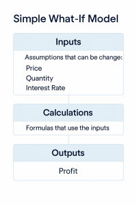
- Use separate areas for:
- Inputs – assumptions that can be changed.
- Calculations – formulas that use the inputs.
- Outputs – results you want to monitor (profit, total cost, balance, etc.).
2. Goal Seek
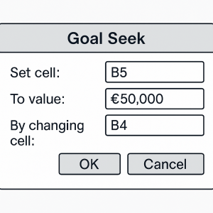
Goal Seek is a what-if tool that works backwards: you specify the result you want, and Excel finds the input value needed to produce that result.
- Use Goal Seek to find the input value needed to reach a target result in a formula cell.
- Example: Find the required sales volume to reach a target profit, by changing units sold while keeping price and cost constant.
- Record and interpret the results:
- Note the changing cell (input), the set cell (result) and the target value.
- Check that the new input is realistic and fits your assumptions.
- Use Goal Seek more than once to test different target values.
3. Scenarios (where supported)
Scenarios allow you to save and switch between sets of input values. This is useful when comparing different options or plans.
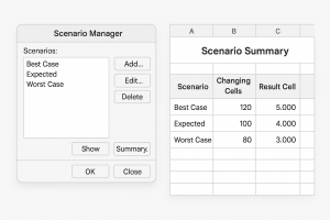
- Create different scenarios such as Best Case, Expected, and Worst Case by changing selected input cells (for example, price, volume, cost).
- Give each scenario a meaningful name and description so it is clear what it represents.
- Switch between scenarios to compare how results (such as profit or balance) change.
- Produce a Scenario Summary report that shows all scenarios side-by-side, including changing cells and result cells.
4. Pivot-style summarising (PivotTables or equivalent)
PivotTables (or equivalent summary tools) let you quickly summarise and analyse large tables of data without changing the original data.
- Create a PivotTable (or equivalent tool) from a well-structured data table with clear headings.
- Drag fields to:
- Rows – categories you want to list down the side (for example, Region, Product).
- Columns – categories you want across the top (for example, Year, Quarter).
- Values – fields you want to summarise (for example, Sum of Sales, Count of Orders).
- Filters – fields you want to filter by (for example, show one Region or Year at a time).
- Summarise data by Sum, Count, Average and other functions as needed.
- Group data, for example by month, quarter, year or by numeric ranges, to make summaries easier to read.

5. Refreshing and managing source data
PivotTables and other summary tools are linked to source data. When the source changes, the summaries need to be refreshed.
- Update the PivotTable or summary when underlying data changes by using the Refresh command.
- Change the source data range if new records are added outside the original range, or base the PivotTable on a table that expands automatically.
- Check that filters, groups and calculation settings are still correct after changing the data source.

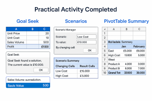
6. Practical Activity
Complete this activity to apply the lesson skills.
Part A – Profit model and Goal Seek
- Build a small profit model with the following inputs and calculations:
- Inputs: Unit Price, Unit Cost, Sales Volume.
- Calculations: Sales = Unit Price × Sales Volume, Total Cost = Unit Cost × Sales Volume, Profit = Sales − Total Cost.
- Use Goal Seek to find the sales volume required to reach a specified profit target (for example, £10,000).
- Note the Goal Seek settings and record the new sales volume required.
Part B – Scenarios
- Using the same model, create at least two scenarios with different cost assumptions, such as:
- Low Cost scenario – reduced Unit Cost.
- High Cost scenario – increased Unit Cost.
- Switch between scenarios to compare the resulting profit.
- Generate a Scenario Summary report showing all scenarios and key results.
Part C – Pivot-style summarising
- In a separate sheet, create or open a small sales table with fields such as Region, Product, Month, Amount.
- Create a PivotTable (or equivalent summary) from the sales table.
- Summarise sales by Region and Product using Sum of Amount.
- Add Month to Columns or Filters and experiment with grouping by month or quarter (where supported).
- Refresh the PivotTable after adding one or two new records to the source data.